5 Conclusion
So far, we have presented a neuro-geometric model for sound reconstruction, proposed an implementation of this model in Julia, and showed results that were published in the GSI 2021 conference proceedings.
In this section we review the model and propose potential routes for future development. We explain as well the faced challenges, the acquired knowledge, and the effect of this internship on my career.
5.1 Reviewing the model
The proposed model has great potential. Upon review, many ideas were sought that are worth exploring, in this section we explain these ideas. These concepts were to be the basis of a PhD project under the supervision of Ugo Boscain, Dario Prandi, and Giuseppina Turco. Unfortunately, we couldn’t receive the funding for a PhD in order to continue working on this fascinating project.
5.1.1 Model analysis
The promising results obtained on simple synthetic sounds, suggested possible applications of the model to the problem of degraded speech [7]. The tests on noisy speech were also promising. However, the tests on cut sound signals were not as impressive. We were prompted to rethink the lift procedure.
In its current situation, the model lifts the time-frequency representation \(S(\tau,\omega)\) of a sound to its time-frequency-chirpiness representation \(L(\tau,\omega,\nu)\) via a heuristic procedure that mimics the naive V1 lift procedure. This presents three main drawbacks:
- The lifted representation \(L(\tau,\omega,\nu)\), which represents the input fed to an A1 neuron \((\omega,\nu)\) at time \(t\), depends strongly on the phase factor of \(S(\tau,\omega)\in\mathbb{C}\). This is unrealistic, since (roughly speaking) the cochlea only transmits the spectrogram \(\left\lvert S(\tau,\omega)\right\rvert\) as A1 is insensitive to phase.
- At a fixed time \(t>0\), the resulting representation \(L(t,\omega,\nu)\) is a distribution, concentrated on a one dimensional curve in the frequency-chirpiness space. This is again unrealistic.
- The current procedure to obtain \(L(\tau,\omega,\nu)\) requires to first compute \(S(\tau,\omega)\) and then to “lift” it. This is not satisfactory from a computational point of view, where one would like to have a streamlined procedure that yield the input \(L\) directly from the original signal.
To improve the model, it is crucial to devise a novel lift procedure allowing to bypass these problems.
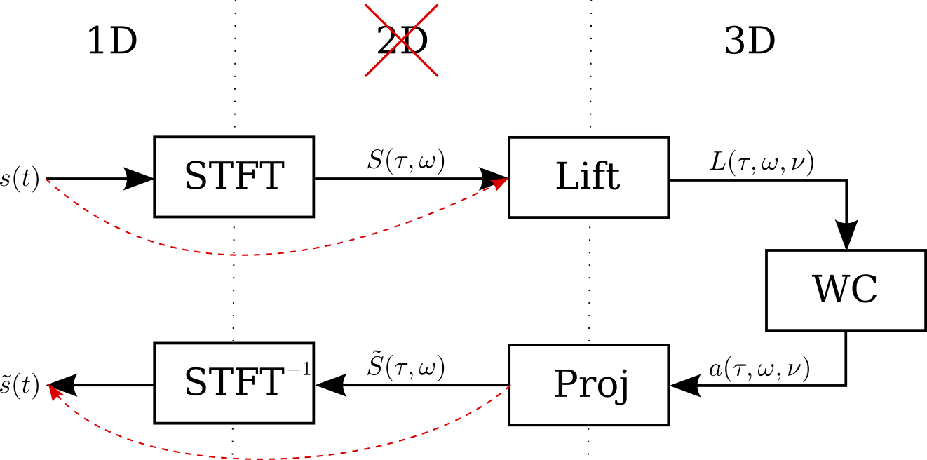
Alternative sound reconstruction pipeline
5.1.2 Wavelet transform
Taking the V1 models as inspiration, it is interesting to apply wavelet analysis techniques in order to construct a reasonable structure for the A1 receptive fields, respecting the symmetries that have already been identified in [7]. This work should be deeply connected with important signal processing concepts, usually applied to the analysis of radar signals [20].
We started reading state-of-the-art literature on the neurophysiology of the inner ear, it was clear that a Wavelet transform represents the signal processing in the cochlea than the STFT transform [24,28]. It is worth mentioning that we studied extensively the auditory representation of acoustic signals by Yang, Wang, and Shamma [28] in order to rethink the model of sound processing in the cochlea.
The Wavelet Transform (WT) of a realizable signal \(s\in L^2(\mathbb{R})\) along a wavelet \(\psi\in L^2(\mathbb{R})\) is defined by
\[\begin{equation} W_\psi s(a,t) = \frac{1}{\sqrt{a}} \int_\mathbb{R}s(\tau) \overline{\psi\left(\frac{\tau-t}{a}\right)} \mathrm{d}\tau \end{equation}\] where \(a\) is the dilation variable.
Generally, the WT has a major advantage over the STFT, which is that the time resolution increases for higher frequencies in the WT.
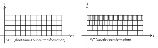
Time resolution in the STFT and the WT [11]
Nevertheless, the WT is given in function of time \(t\) and the dilation variable \(a\). While \(a\) implicitly represents the frequency, obtaining the chirpiness is not as straightforward as in the case of the STFT. In fact, we haven’t been able to define an appropriate lift from the WT. However, the WT represents a path worth exploring more for improving the model.
5.1.3 The lift operator
We have seen the definition of the STFT operator \(V_\gamma\) in equation () from unitary time and frequency shift operators \(T_\tau,M_\omega\in\mathcal{U}(L^2(\mathbb{R}))\). A mathematically elegant solution to the lift problem is to introduce a unitary operator \(C_\nu\) on realizable signals \(s\in L^2(\mathbb{R})\) such that
\[\begin{equation} L_\gamma s(\tau,\omega,\nu) = \left\langle s,C_\nu M_\omega T_\tau \gamma\right\rangle_{L^2(\mathbb{R})} \end{equation}\]
such an operator would be mathematically stable and computationally cheap. Unfortunately, no such result was obtained, only further exploration would reveil if such representation is possible.
5.1.4 The group representation
The quest of redefining the sound lift to the contact space from the Wavelet transform time-frequency representation started by studying the group representation of the model.
Developing the group representation of the time-frequency representation ended up confirming both models. Unfortunately, the work didn’t result in a mathematical definition of the chirpiness (see Appendix C). Nevertheless, the established work would serve as a basis for further exploration.
5.1.5 The WCA1.jl package
The new implementation qualifies as a Julia package, given the quality of the code with respect to efficiency and its documentation.
Hence, once the model is adjusted, the resulting code should be released
as a free open-source Julia package.
Which would contribute to the quite immature sound signal processing ecosystem
in Julia (alongside DSP.jl and WAV.jl).
Finally, the resulting code should be published on JOSS (the Journal of Open Source Software).
5.1.6 A sparse lift implementation
I noticed that the lifted sound representation \(L[\tau,\omega,\nu]\) was sparse 3D array. This quality would save a lot of memory since in our samples the ratio of non-zero elements in \(L\) was under \(10\%\).
Nevertheless, Julia does not have a standard implementation for sparse 3D arrays.
I therefore proceeded to research and implement a hashmap-based (dictionary) sparse 3D array
on top of Julia’s standard AbstractSparseArray interface.
My implementation would occupy under \(15\%\) of the memory.
However, the computation speed is considerably less as the hashmap-based approach
for encoding sparse 3D arrays is far from optimal.
An alternative more efficient approach could be considered for implementing such module
without compromising the algorithm’s speed.
5.2 Acquired knowledge
The presented model is clearly complex and interdisciplinary. The mission requires a deep understanding of fundamental mathematics, namely geometry, control theory, and group representations, as well as applied mathematics skills such as signal processing and numerical analysis.
While the general mission of the internship was known beforehand, the tasks I had to carry out where changed in light of new results and my role evolved throughout the internship.
I first needed to familiarize myself with the accomplished work, a preliminary study of the image reconstruction was needed in order to understand the sound model and the challenges that are faced in adapting the initial model for sound reconstruction. This triggered learning new mathematical concepts. I did a general reading of Foundations of Time-Frequency Analysis by Gröchenig [15] which served as a reference throughout the internship. While I had a working understanding of basic Fourier analysis thanks to INSA courses and a familiarity of the Uncertainty Principle and the Short-Time Fourier Transform thanks to my work on music information retreival for my final Master’s project. The book explains these principles rigourously and also serves as a great source for learning about the Heisenberg Group and Wavelet Transforms which are the basis of the proposed model.
Moreover, studying the existing litterature on the subject and working the mathematical model helped me learn domains of fundamental and applied mathematics that were new to me.
In addition, co-writing a conference paper and attending the conference of Geometric Science of Information was an outstanding experience that I am for extremely grateful.
Finally, the model is implemented in Julia code, which was a new programming language for me, I therefore learned Julia to be able to improve the existing code. Having a great basis in low-level and high-level languages, undoubtedly due to my INSA education and internships, I was able to write Julia code in very little time. Nevertheless, it was very important to me to learn Julia norms and common practices to write elegant and modular code, as well as learning the mechanisms of this high-level language in order to optimize the code’s performance. This deeper knowledge of Julia was gained in the following months.
5.3 My future project
This internship has widened my horizons even more than I had hoped. I have been more and more interested in pursuing a career in academic research for the last few years. Nevertheless, this internship has allowed me to confirm my interest in such career. I also gained an appreciation for geometry and analysis.
While I didn’t get the opportunity to pursue a PhD thesis in this project, I have decided, with the help and guidance of my supervisors, to enroll in a theoretical mathematics Master’s degree at University of Lorraine in Nancy. The program focuses on PDEs and control theory from a theoretical point of view, which would allow me, combined with my skills in applied mathematics that I cultivated at INSA Rouen Normandie, to pursue a PhD in these domains.