3 Sound reconstruction model
3.1 From V1 to A1
The motivation behind the application of the model in sound reconstruction is the idea that a sound can be seen as an image in the time-frequency domain. The primary auditory cortex A1 receives the sensory input directly from the cochlea [12], which is a spiral-shaped fluid-filled cavity that composes the inner ear.
The mechanical vibrations along the basilar membrane are transduced into electrical activity along a dense, topographically ordered, array of auditory-nerve fibers which convey these electrical potentials to the central auditory system.
Since these auditory-nerve fibers (sensors or inner hair cells) are topographically ordered along the cochlea spiral, different regions of the cochlea are sensitive to different frequencies. Hair cells close to the base are more sensitive to low-frequency sounds and those near the apex are more sensitive to high-frequency sounds [28].
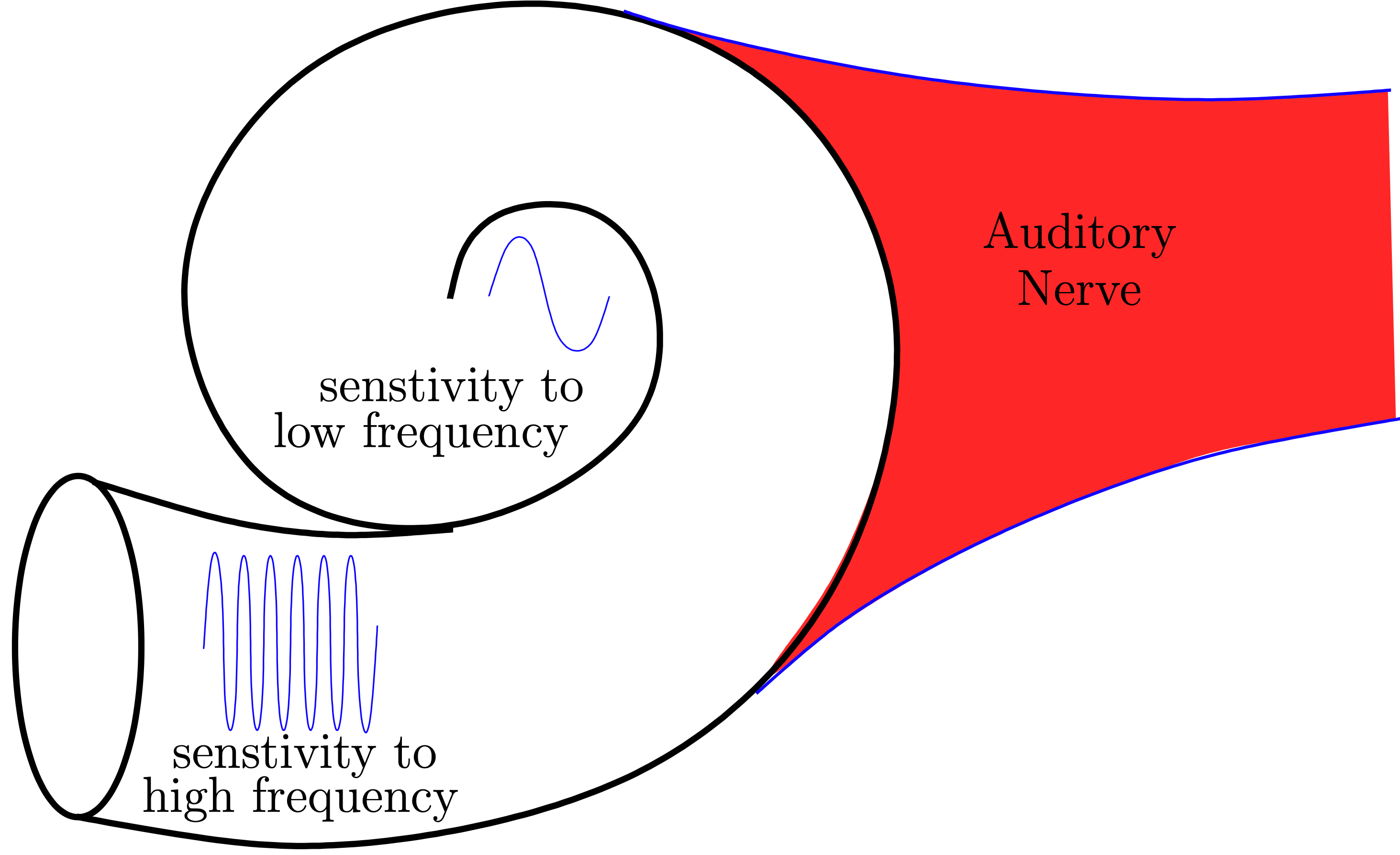
Perceived pitch of a sound depends on the location in the cochlea that the sound wave stimulated [7].
This spatial segregation of frequency sensitivity in the cochlea means that the primary auditory cortex receives a time-frequency representation of the sound. In this model, we consider the Short-Time Fourier Transform (STFT) as the time-frequency representation \(S(\tau,\omega)\) of a sound signal \(s\in L^2(\mathbb{R})\)
While the spectrogram of a sound signal \(\left\lvert S\right\rvert(\tau,\omega)\) is an image, the image reconstruction algorithm cannot be applied to a corrupted sound since the rotated spectrogram would correspond to completely different input sound therefore the invariance by rototranslation is lost. Moreover, the image reconstruction would evolve the WC equation on the entire image simultaneously. However, the sound image (spectrogram) does not reach the auditory cortex simultaneously but sequentially. Hence, the reconstruction can be performed only in a sliding window [7].
3.2 Sound reconstruction pipeline
As discussed in the previous section, the sound reconstruction model is inspired by the V1 model. First, a 2-dimensional image of the sound signal is obtained via a short-time Fourier transform, which is analogous to the spectrogram the cochlea transmits to the auditory cortex. The time derivative of the frequency \(\nu=\mathrm{d}\omega/\mathrm{d}\tau\), corresponding to the chirpiness of the sound, allows adding a new dimension to the sound image. Afterwards, the sound image is lifted into an augmented space that is \(\mathbb{R}^3\) with the Heisenberg group structure. Henceforth, the sound is processed in its 3D representation, that is the obtained lift \(L(\tau,\omega,\nu)\).
Similarly to the V1 model, the sound is reconstructed by solving the Wilson-Cowan integro-differential equation.
Finally, the solution to the Wilson-Cowan equations is projected into the time-frequency representation which gives a sound signal through an inverse short-time Fourier transform [7].
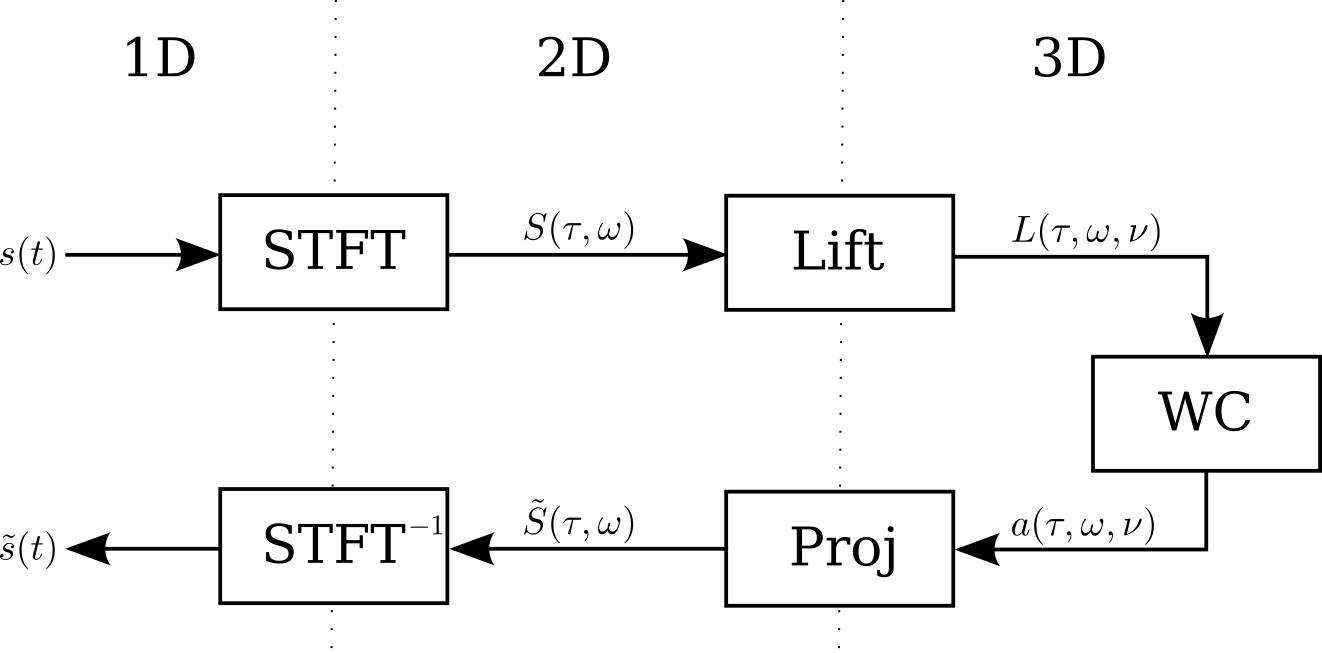
Sound reconstruction pipeline
3.3 Time-Frequency representation
The Fourier transform transforms a time signal \(s\in L^2(\mathbb{R})\) into a complex function of frequency \(\hat s\in L^2(\mathbb{R})\). Since the time signal \(s\) can be obtained from \(\hat s\) using the Inverse Fourier Transform, they both contain the exact same information. Conceptually, \(s\) and \(\hat s\) can be considered two equivalent representations of the same object \(s\), but each one makes visible different features of \(s\).
A time-frequency representation would combine the features of both \(s\) and \(\hat s\) into a single function. Such representation provides an instantaneous frequency spectrum of the signal at any given time [15].
3.3.1 The Short-Time Fourier Transform
The Short-Time Fourier Transform (STFT) is a very common Time-Frequency representation of a signal. The principle of the STFT is quite straightforward. In order to obtain a Time-Frequency representation of a signal \(s\), a Fourier transform is taken over a restricted interval of the original signal sequentially. Since a sharp cut-off introduces discontinuities and aliasing issues, a smooth cut-off is prefered [15]. This is established by multiplying a segment of the signal by a weight function, that is smooth, compactly supported, and centered around \(0\), referred to as window. Essentially, the STFT \(S(\tau,\omega)\) is the Fourier transform of \(s(t)w(t-\tau)\) (the signal taken over a sliding window along the time axis.)
\[\begin{equation} S(\tau,\omega) = \int_\mathbb{R}s(t)w(t-\tau)e^{-2\pi i\omega t} \mathrm{d}t \end{equation}\]
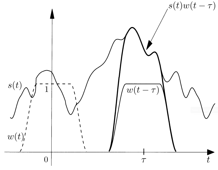
Signal windowing for the STFT [15]
3.3.2 Time and frequency shifts operators
In our study, we consider realizable signals \(s\in L^2(\mathbb{R})\). Fundamental operators in time-frequency analysis are time and phase shifts acting on realizable signals \(s\in L^2(\mathbb{R})\).
- Time shift operator: \(T_\tau s(t)=s(t-\tau)\)
- Phase shift operator: \(M_\omega s(t)=e^{2\pi i \omega t} s(t)\)
We notice that the STFT can be formulated using these unitary operators
\[\begin{align} S(\tau,\omega) &= \int_\mathbb{R}s(t)w(t-\tau)e^{-2\pi i\omega t} \mathrm{d}t\\ &= \int_\mathbb{R}s(t) \overline{M_\omega T_\tau w(t)} \mathrm{d}t\\ &= \left\langle s, M_\omega T_\tau w\right\rangle_{L^2(\mathbb{R})} \end{align}\]
We can redefine the STFT as an operator \(V_w\) on \(s\in L^2(\mathbb{R})\) defined in function of \(T_\tau\) and \(M_\omega\) [7,15].
\[\begin{equation}\label{eq:stft_operator} V_w s(\tau,\omega) = \left\langle s, M_\omega T_\tau w\right\rangle_{L^2(\mathbb{R})} \end{equation}\]
3.3.3 Discrete STFT
Similarly to the continuous STFT, the discrete STFT is the Discrete Fourier Transform (DFT) of the signal over a sliding window. Nevertheless, the window cannot slide continuously along the time axis, instead the signal is windowed at different frames with an overlap. The window therefore hops along the time axis.
Let \(N\) be the window size (DFT size), we define the overlap \(R\) as the number of overlapping frames between two consecutive windows. The hop size is therefore defined as \(H=N-R\). We also define the overlap ratio as the ratio of the overlap with respect to the window size \(r=R/N\) where \(r\in[0,1[\).
The discrete STFT of a signal \(s\in L^2([0,T])\) is therefore \[\begin{equation} S[m,\omega] = \sum_{t=0}^{T} s[t]w[t-mH]e^{-2\pi i\omega t} \end{equation}\]
The choice of parameters has direct influence over the discrete STFT resolution, as well as its invertibility.
3.3.4 STFT windowing
The choice of the window affects quality of the Fourier transform. One should choose a window with anti-aliasing and that distributes spectral leakage.
(a) Rectangular window
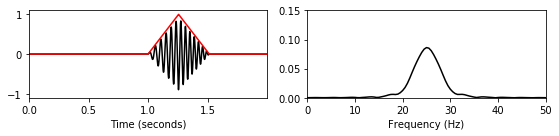
(b) Triangular window
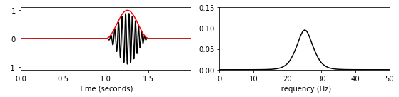
(c) Hann window
Different windows (left) and their respective Fourier transform (right)
Moreover, as we will see in the next sections, the STFT is invertible. However, the STFT parameters need to satisfy the two following constraints [14,21]:
- Nonzero OverLap Add (NOLA): \(\sum\limits_{m\in\mathbb{Z}} w^2[t-mH] \neq 0\)
- Constant OverLap Add (COLA): \(\sum\limits_{m\in\mathbb{Z}} w[t-mH] = 1\)
The NOLA condition is met for any window given an overlap ratio \(r\in[0,1[\). It is worth noting that this condition can be found without the square depending on the inverse STFT algorithm.
The COLA constraint defines the partition of unity over the discrete time axis, imposing a stronger condition.
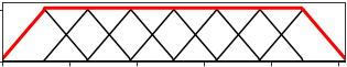
(a) Triangular window, overlap ratio \(r=\frac{1}{2}\)
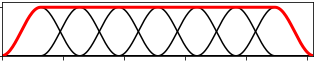
(b) Hann window, overlap ratio \(r=\frac{1}{2}\)
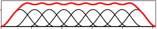
(c) Hann window, overlap ratio \(r=\frac{3}{8}\)
The COLA condition with different windows and overlap ratios
In typical applications, the window functions used are non-negative, smooth, bell-shaped curves [25]. A comprehensive list of windows and their properties may be found in [16]. In our model we use the Hann window, which satisfies the COLA condition for any overlap ratio of \(r=\frac{n}{n+1},n\in\mathbb{N}^*\).
The Hann window of length \(L\) is defined as \[\begin{equation} w(x)=\begin{cases} \frac{1+\cos\left(\frac{2\pi x}{L}\right)}{2} & \text{if}~\left\lvert x\right\rvert\leq\frac{L}{2}\\ 0 & \text{if}~\left\lvert x\right\rvert>\frac{L}{2} \end{cases} \end{equation}\]
3.3.5 Uncertainty principle and resolution issues
As previously stated, both \(s\) and \(\hat s\) contain the exact same information. However, there is a fundamental limit to the accuracy with which the values for certain pairs of physical pairs can be observed. A known example to issue is Heisenberg’s uncertainty principle regarding the position of a particle and its momentum [26]. Similarly, time and frequency are a pair of complementary variables.
In the context of time-frequency analysis, the Heisenberg-Gabor limit (or simply the Gabor limit) defines this constraint by the following inequality (proof in Appendix B)
\[\begin{equation} \sigma_t\cdot\sigma_\omega\geq \frac{1}{4\pi} \end{equation}\] where \(\sigma_t\) and \(\sigma_\omega\) are the standard deviations of the time and frequency respectively.
The Gabor limit means essentially that “a realizable signal occupies a region of area at least one in the time-frequency plane.” Which means that we cannot sharply localize a signal in both the time domain and frequency domain. This makes the concept of an instantaneous frequency impossible [15].
A direct result of the uncertainty principle is the fact that high temporal resolution and frequency resolution cannot be acheived at the same time.
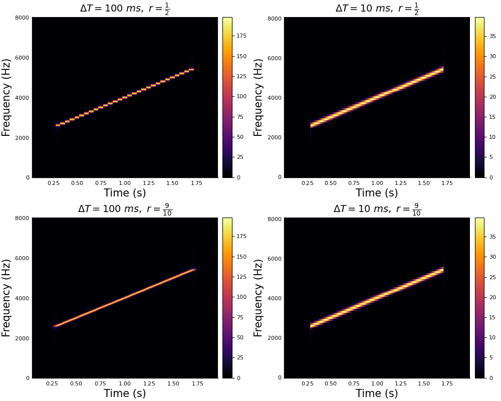
STFT resolution with respect to different window sizes \(\Delta T\) and overlap ratios \(r\)
In the figure above, we see the influence of the window size and the overlap ratio on the STFT resolution.
- Window size: For larger window sizes, we have higher frequency resolution. However, the time resolution is low as we have fewer time samples for the STFT. For smaller windows, we get higher time resolution as we have more time samples for the STFT, while losing frequency resolution due to smaller FT size.
- Overlap: In the case of smaller overlaps, the resulting spectrum has time discontinuities. Indeed, the straight line appears to be a piece-wise constant function of time. For overlap ratios close to 1, the time resolution is significantly better obtaining the best results (given an adequate window size). However, one should keep in mind that high overlaps can be computationally costly.
3.3.6 Inverse Short-Time Fourier Transform
The operator \(V_w\) is an isometry from \(L^2(\mathbb{R})\) to \(L^2(\mathbb{R}^2)\) if \(\left\lVert w\right\rVert_2=1\), allowing for \(s\) to be completely determined by \(V_w s\). With the help of the orthogonality relations (Parseval’s formula) on the STFT we obtain the inversion formula for the STFT (see Appendix A for a detailed proof).
For \(w,h\in L^2(\mathbb{R})\) smooth windows such that \(\left\langle w,h\right\rangle\neq 0\) we have for all \(s\in L^2(\mathbb{R})\),
\[\begin{align} s(t) &=\frac{1}{\left\langle w,h\right\rangle} \iint_{\mathbb{R}^2}V_w s(\tau,\omega)M_\omega T_\tau h(t) \mathrm{d}\omega\mathrm{d}\tau\\ &= \frac{1}{\left\langle w,h\right\rangle} \iint_{\mathbb{R}^2} S(\tau,\omega) h(t-\tau) e^{2\pi i\omega t} \mathrm{d}\omega\mathrm{d}\tau \end{align}\]
3.3.7 Griffin-Lim Algorithm
The practical use of the inverse STFT is to obtain the signal from a spectrum that has undergone some changes. Daniel W. Griffin and Jae S. Lim [14] proposed an efficient algorithm for signal estimation from the modified STFT. The GLA algorithm minimizes the mean squared error between the STFT magnitude of the estimated signal and the modified STFT magnitude.
This method is efficient and easy to implement, and is widely used in signal processing libraries.
Let \(x\in L^2(\mathbb{R})\) be a realizable signal and \(X=V_w x\in L^2(\mathbb{R}^2)\) be its STFT. Let \(Y\in L^2(\mathbb{R}^2)\) denote the modified STFT. It’s worth noting that \(Y\), in general, is not necessarily an STFT in the sense that there might not be a signal \(y\in L^2(\mathbb{R})\) whose STFT is \(Y=V_w y\) [14].
Let \(y_\tau \in L^2(\mathbb{R}^2)\) the inverse Fourier transform of \(Y\) with respect to the frequency \(\omega\) (its second variable) at a fixed time \(\tau\in\mathbb{R}\).
\[\begin{equation} y_\tau(t) = \int_{\mathbb{R}} Y(\tau,\omega) e^{2\pi i\omega t} \mathrm{d}\omega \end{equation}\]
The algorithm finds iteratively the signal \(x\) that minimizes the distance between \(X\) and \(Y\). The distance measure between the two spectrums is defined as the norm of the difference over the \(L^2(\mathbb{R}^2)\) space
\[\begin{equation} d(X,Y) = \left\lVert X-Y\right\rVert_2^2 = \iint_{\mathbb{R}^2} \left\lvert X(\tau,\omega) - Y(\tau,\omega)\right\rvert^2 \mathrm{d}\omega\mathrm{d}\tau \end{equation}\]
Which is expressed for discrete STFT as \[\begin{equation} d(X,Y) = \sum_\tau \sum_\omega\left\lvert X[\tau,\omega] - Y[\tau,\omega]\right\rvert^2 \end{equation}\]
The signal \(x[t]\) is therefore reconstructed iteratively along the formula \[\begin{equation} x[t] = \frac{\sum\limits_\tau y_\tau[t]w[t-\tau]}{\sum\limits_\tau w^2[t-\tau]} \end{equation}\]
3.4 The lift to the augmented space
In order to study the Wilson-Cowan model for neural activations, we need to have a 3D representation of the sound. In this section we will explain how the STFT of the sound signal is lifted into the contact space and explore the properties of this space.
3.4.1 The sound chirpiness
The 3D representation of the image in the sub-Riemannian model of V1 was obtained by considering the sensitivity to directions represented by an angle \(\theta\in P^1=\mathbb{R}/\pi\mathbb{Z}\).
We transpose this concept of sensitivity to directions for sound signals to sensitivity to instantaneous chirpiness that is the time derivative of the frequency \(\nu=\mathrm{d}\omega/\mathrm{d}\tau\). The time derivative of the frequency is indeed the slope of the tangent line in the sound spectrogram. Hence establishing the bridge with the visual model.
3.4.2 Single time-varying frequency
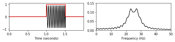
As we study the sound through its instantaneous frequency and chirpiness, we consider both the frequency and the chirpiness functions of time. To properly define the lift, we consider the following single time-varying frequency sound signal
\[\begin{equation} s(t) = A\cdot\sin(\omega(t)t),\quad A\in\mathbb{R} \end{equation}\]
The STFT of this signal can be therefore expressed as
\[\begin{equation} S(\tau,\omega) = \frac{A}{2i}\left(\delta_0(\omega-\omega(\tau)) - \delta_0(\omega+\omega(\tau))\right) \end{equation}\]
supposing the FT is normalized, where \(\delta_0\) is the Dirac delta distribution centered at 0. Which means that \(S\) is concentrated on the curves \(\tau\mapsto(\tau,\omega(\tau))\) and \(\tau\mapsto(\tau,-\omega(\tau))\).
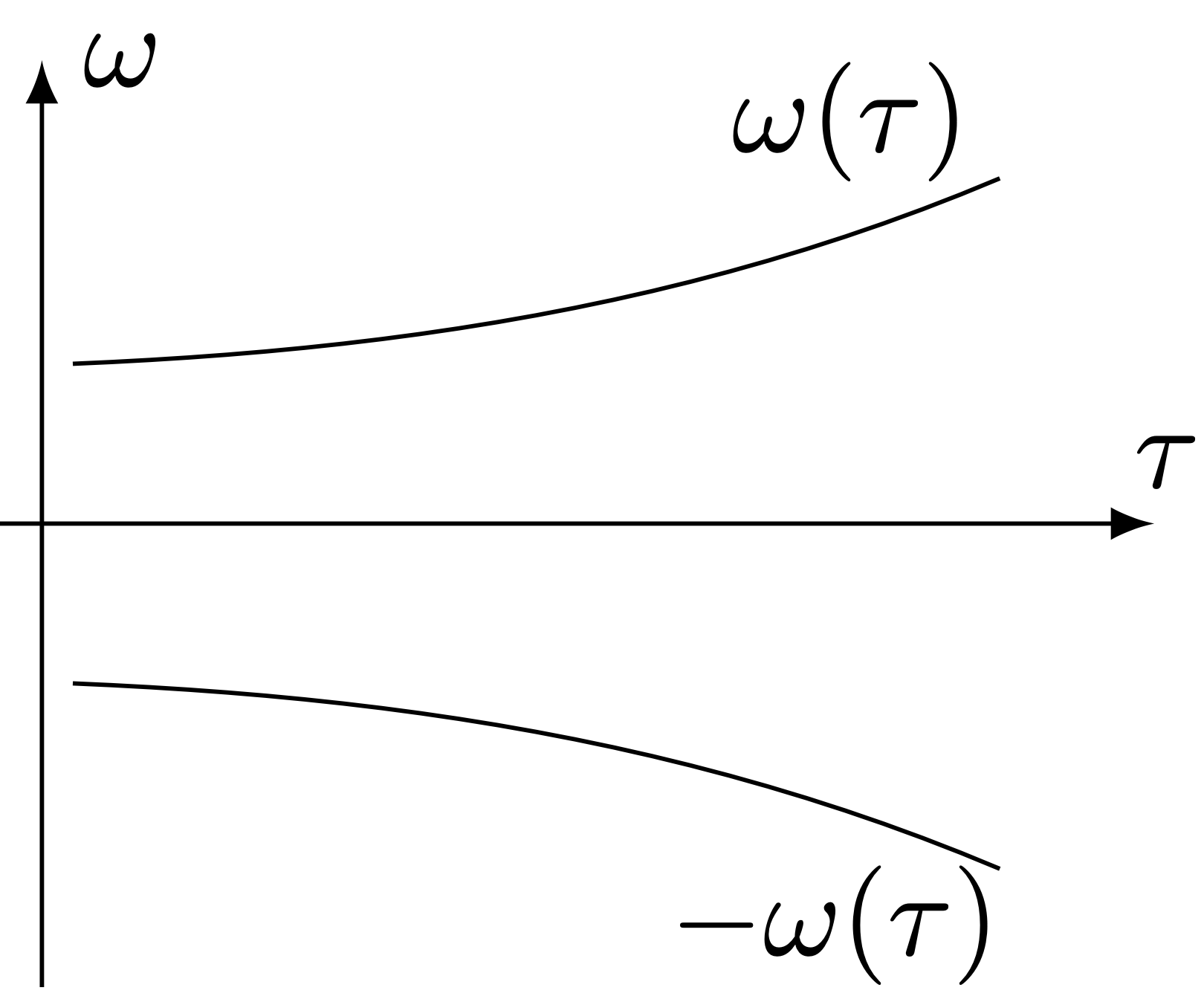
The STFT the single time-varying frequency sound signal
So far, the sound signal is represented in the 2-dimensional space by the parametric curve \(t\mapsto(t,\omega(t))\). Nevertheless, we aim to lift our signal into the 3-dimensional augmented space by adding the sensitivity to frequency variations \(\nu(t)=\mathrm{d}\omega(t)/\mathrm{d}t\). Similarly, the lifted curve is parameterized as \(t\mapsto(t,\omega(t),\nu(t))\) [7].
3.4.3 Control system
We define the control to the chirpiness variable \(u(t)=\mathrm{d}\nu/\mathrm{d}t\), we can therefore say that the curve \(t\mapsto(\tau(t),\omega(t),\nu(t))\) in the contact space is a lift of a planar curve if there exists a control \(u(t)\) such that
\[\begin{equation} \frac{\mathrm{d}}{\mathrm{d}t}\begin{pmatrix}\tau\\\omega\\\nu\end{pmatrix} = \begin{pmatrix}1\\\nu\\0\end{pmatrix} + u(t)\begin{pmatrix}0\\0\\1\end{pmatrix} \end{equation}\]
We define the system state vector as \(q=(\tau,\omega,\nu)\), the control system can be written as \[\begin{equation} \frac{\mathrm{d}}{\mathrm{d}t}q(t) = X_0(q(t)) + u(t) X_1(q(t)) \end{equation}\]
where \(X_0(q(t))\) and \(X_1(q(t))\) are two vector fields in \(\mathbb{R}^3\) defined as
\[\begin{equation} X_0\begin{pmatrix}\tau\\\omega\\\nu\end{pmatrix} = \begin{pmatrix}1\\\nu\\0\end{pmatrix},\quad X_1\begin{pmatrix}\tau\\\omega\\\nu\end{pmatrix} = \begin{pmatrix}0\\0\\1\end{pmatrix} \end{equation}\]
The vector fields \(X_0\) and \(X_1\) generate the Heisenberg group, and the space \(\left\{X_0+uX_1\vert u\in\mathbb{R}\right\}\) is a line in the \(\mathbb{R}^3\) [7].
3.4.4 Lift to the contact space
In the case of a general sound signal, each level line of the spectrogram \(\left\lvert S\right\rvert(\tau,\omega)\) is lifted to the contact space. This yeilds by the implicit function theorem the following subset of the contact space, which is a well-defined surface if \(\left\lvert S\right\rvert\in\mathcal{C}^2\) and \(\mathrm{Hess}\left\lvert S\right\rvert\) is non-degenerate [7].
\[\begin{equation} \Sigma = \left\{(\tau,\omega,\nu)\in\mathbb{R}^3 \vert\nu\partial_\omega\left\lvert S\right\rvert(\tau,\omega) + \partial_\tau\left\lvert S\right\rvert(\tau,\omega) = 0\right\} \end{equation}\]
Which allows to finally define the sound lift in the contact space as
\[\begin{equation} L(\tau,\omega,\nu) = S(\tau,\omega)\cdot\delta_\Sigma (\tau,\omega,\nu) = \begin{cases} S(\tau,\omega) & \text{if}~(\tau,\omega,\nu)\in\Sigma\\ 0 & \text{otherwise} \end{cases} \end{equation}\]
The time-frequency representation is obtained from the lifted sound by applying the projection operator defined as
\[\begin{equation} \mathrm{Proj}\left\{L(\tau,\omega,\nu)\right\}(\tau,\omega) = \int_\mathbb{R}L(\tau,\omega,\nu)\mathrm{d}\nu \end{equation}\]
3.4.5 Lift implementation
We have seen that the lift to the contact space is defined through the surface \(\Sigma\) which is defined with respect to \(\nabla\left\lvert S\right\rvert\). The chirpiness is numerically calculated by numerically approximating the gradient of the spectrum \(\left\lvert S\right\rvert\).
The discretization of the time and frequency domains is determined by the sampling rate of the original signal and the window size chosen in the STFT procedure. That is, by the Nyquist-Shannon sampling theorem, for a temporal sampling rate \(\delta t\) and a window size of \(T_w\), we consider the frequencies \(\omega\) such that \(|\omega|<1/(2\delta t)\), with a finest discretization rate of \(1/(2T_w)\).
The frequency domain is therefore bounded. Nevertheless, the chirpiness \(\nu\) defined as \(\nu\partial_\omega\left\lvert S\right\rvert(\tau,\omega) + \partial_\tau\left\lvert S\right\rvert(\tau,\omega)=0\) is unbounded, and since generically there exists points such that \(\partial_\omega\left\lvert S\right\rvert(\tau_0,\omega_0)=0\), chirpiness values stretch over the entire real line.
To overcome this problem, a natural strategy is to model the chirpiness values as a random variable \(X\), and considering only chirpinesses falling inside the confidence interval \(I_p\) for some reasonable \(p\)-value (e.g., \(p=0.95\)). The best fit for the chirpiness values was the random variable \(X\) following a Cauchy distribution \(\mathrm{Cauchy}(x_0,\gamma)\) [4] where
- \(x_0\) is the location parameter that corresponds to the location of the peak
- \(\gamma\) is the scale parameter that determines the shape of the distribution
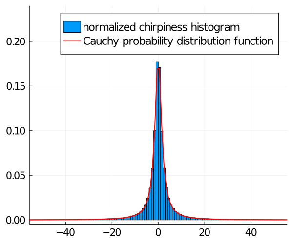
Chirpiness of a speech signal compared to Cauchy distribution
The Cauchy distribution’s probability density function (PDF) is given as \[\begin{equation} f_X(x)=\frac{1}{\pi\gamma\left(1+\left(\frac{x-x_0}{\gamma}\right)^2\right)} \end{equation}\] and it’s cumulative distribution function (CDF) is \[\begin{equation} F_X(x)=\frac{1}{\pi} \arctan\left(\frac{x-x_0}{\gamma}\right) + \frac{1}{2} \end{equation}\]
The Cauchy parameters were estimated as follows:
- \(x_0\): the chirpiness samples median
- \(\gamma\): half the interquartile range which is the difference between the 75th and the 25th percentile.
Although statistical tests on a library of real-world speech signals1 rejected the assumption that \(X\sim \mathrm{Cauchy}(x_0,\gamma)\), the fit is quite good according to the Kolmogorov-Smirnov statistic \[\begin{equation} D_n=\sup_x\left\lvert F_n(x)-F_X(x)\right\rvert \end{equation}\] where \(F_n\) is the empirical distribution function evaluated over the chirpiness values [4].
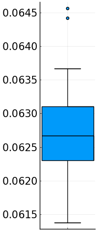
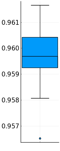
Box plots for estimated Cauchy distributions of speech signals chirpiness. Left: Kolmogorov-Smirnov statistic values. Right: percentage of values falling in \(I_{0.95}\)
3.5 Cortical activations in A1
In this model, we consider the primary auditory cortex (A1) as the space of \((\omega,\nu)\in\mathbb{R}^2\). When hearing a sound signal \(s\), A1 receives its lift to the contact space \(L(t,\omega,\nu)\) at every instant \(t\). The neuron receives an external charge \(S(t,\omega)\) if \((t,\omega,\nu)\in\Sigma\) and no charge otherwise.
The Wilson-Cowan equations (WC) [27] have been successfully applied to describe the evolution of neural activations in V1 as well as A1 [5,6,9,13,19,23,29].
The WC equations have the advantage of being flexible as they can be applied independently of the underlying geometric structure, which is only encoded in the kernel of the integral term. They allow as well for a natural implementation of delay terms in the interactions and can be easily tuned via few parameters with clear effect on the results.
In this model, the resulting activation \(a:[0,T]\times\mathbb{R}\times\mathbb{R}\rightarrow\mathbb{C}\) is the solution to the WC differo-integral equation with a delay \(\delta\).
\[\begin{equation} \frac{\partial}{\partial t}a(t,\omega,\nu) = -\alpha a(t,\omega,\nu) + \beta L(t,\omega,\nu) + \gamma\int_{\mathbb{R}^2} k_\delta(\omega,\nu\Vert\omega',\nu') \sigma(a(t-\delta,\omega',\nu')) \mathrm{d}\omega'\mathrm{d}\nu' \end{equation}\]
where
- \(\alpha,\beta,\gamma>0\) are parameters
- \(\sigma:\mathbb{C}\rightarrow\mathbb{C}\) is a non-linear sigmoid where \(\sigma(\rho e^{i\theta})=\tilde\sigma(\rho)e^{i\theta}\) with \(\tilde\sigma(x)=\min\left\{\max\left\{0,\kappa x\right\}, 1\right\},\forall x\in\mathbb{R}\) given a fixed \(\kappa>0\).
- \(k_\delta(\omega,\nu\Vert\omega',\nu')\) is a weight modeling the interaction between \((\omega,\nu)\) and \((\omega',\nu')\) after a delay \(\delta>0\) via the kernel of the transport-diffusion operator associated to the contact structure of A1.
When \(\gamma=0\), the WC equation becomes a standard low-pass filter \(\partial_t a=-\alpha a + L\) whose solution is simply
\[\begin{equation} a(t,\omega,\nu) = \int_0^t e^{-\alpha(s-t)}L(t,\omega,\nu)\mathrm{d}s \end{equation}\]
With \(\gamma\neq0\), a non-linear delayed interaction term is added on top of the low-pass filter, encoding the inhibitory and excitatory interconnections between neurons [7].
In the scope of the internship, no work was carried on the integral kernel. Hence, no further explanation on the WC model is needed.
References
The speech material used in the current study is part of an ongoing psycholinguistic project on spoken word recognition. Speech material comprises 49 Italian words and 118 French words. The two sets of words were produced by two (40-year-old) female speakers (a French monolingual speaker and an Italian monolingual speaker) and recorded using a headset microphone AKG C 410 and a Roland Quad Capture audio interface. Recordings took place in the soundproof cabin of the Laboratoire de Phonétique et Phonologie (LPP) of Université de Paris Sorbonne-Nouvelle. Both informants were told to read the set of words as fluently and naturally as possible↩︎