4 Implementation
Julia is a relatively new language, it first appeared in 2012, and its version 1.0 was released in 2018. The language was built to be fast, general-purpose, dynamic, and highly technical [3].
Julia respresents a great alternative for scientific computing and visualization to replace C/C++, Fortran, Python, Matlab, and R. It is designed to have the speed of C and Fortran, with the ease of use of Python, Matlab, and R. All while maintaining a great syntax for general purpose programming.
Julia is a serious contender as a scientific programming language. However, the Julia community is still considerabely smaller than other scientific programming languages. For instance, in the 2021 Stack Overflow Developer Survey, 1.29% responded they wanted to work in Julia over the next year against 48.24% in Python and 4.66% in Matlab [1]. As a result, Julia has less stable scientific libraries than other languages.
4.1 The WCA1.jl library
The model was first implemented by Dario Prandi,
allowing to present a series of experiments on simple synthetic sounds.
The code and the experiments are available at
https://github.com/dprn/WCA1.
The work I carried on during the internship was built on top of the original code,
my contributions are available at
https://github.com/rand-asswad/WCA1,
which is forked from the original repository.
Indeed, rewriting the code was necessary in order to experiment on real sound signals as they are considerabely larger, otherwise the code would run for a long time and in some cases errors would arise. Moreover, an official scientific package should be well-written and well-documented, and should also try to respect Julia’s code style and recommendations.
4.1.1 The STFT module
Reimplementing the STFT module was necessary in order to carry out
experiments on real sound signals, the preexisting code was not well
adapted for such signals.
Furthermore, an inverse STFT implementation is missing from the Julia
standard libraries such as FFTW.jl
and DSP.jl.
Hence, I researched efficient algorithms for implementing the inverse STFT
and landed on the Griffin-Lim algorithm [14].
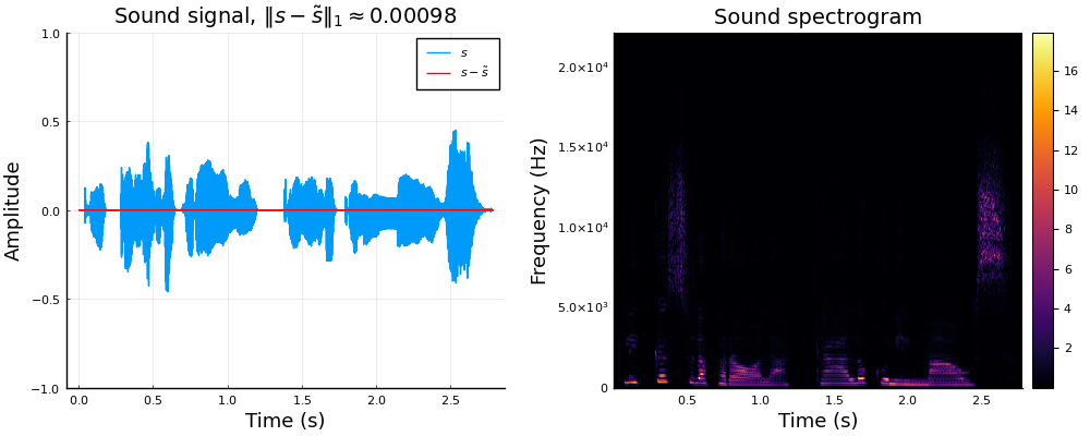
Left: speech sound \(s\) compared with \(\tilde s=\mathrm{STFT}^{-1}\left\{\mathrm{STFT}\left\{s\right\}\right\}\). Right: spectrogram \(\left\lvert S\right\rvert(\tau,\omega)=\left\lvert\mathrm{STFT}\left\{s(t)\right\}\right\rvert\)
4.1.2 Optimizing the lift module
The sound chirpiness is computed by calculating gradient of the spectrum matrix \(\nabla\left\lvert S\right\rvert\), which gives the chirpiness with respect to each time-frequency pair
\[\begin{equation} \nu(\tau,\omega) = \begin{cases} -\frac{\partial_\tau\left\lvert S\right\rvert(\tau,\omega)}{\partial_\omega\left\lvert S\right\rvert(\tau,\omega)} & \text{if}~\left\lvert\partial_\omega\left\lvert S\right\rvert(\tau,\omega)\right\rvert>\varepsilon\\ 0 & \text{otherwise} \end{cases} \end{equation}\]
where \(\varepsilon\) is a small threshold.
Afterwards, the chirpiness values are compared to a Cauchy distribution, allowing to establish a confidence interval \(I_p\) (we take \(p=0.95\)), in order to cut the tails that extend over the entire real line.
The chirpiness values \(\nu\in I_p=[\nu_{\min},\nu_{\max}]\) are then discretized as the following: Let \((\nu_n)_{1\leq n\leq N}\) such that \(\nu_{\min}=\nu_1<\cdots<\nu_N=\nu_{\max}\). Each value \(\nu\) is rounded to the nearest \(\nu_n\).
\[\begin{equation} n(\nu) = \left\lfloor\frac{\nu - \nu_{\min}}{\nu_{\max}- \nu_{\min}}(N-1) + 1\right\rceil,\quad\forall\nu\in I_p \end{equation}\] where \(\left\lfloor\cdot\right\rceil:\mathbb{R}\rightarrow\mathbb{Z}\) is the rounding function to the nearest integer.
This was optimized by implementing the function in a variety of ways, then benchmarking the time and memory consumption for each implementation over every sample sound from the speech library. We noticed that the rounding function \(n(\nu)\) can be rewritten as an affine function with respect to \(\nu\), avoiding to do the same operations inside the loop, thus saving time and memory. The explicit expression and the affine expression were both implemented using a traditional loop, list comprehension, and Julia’s broadcast operator. The list comprehension was clearly the fastest, without compromising the function’s readability nor memory consumption.
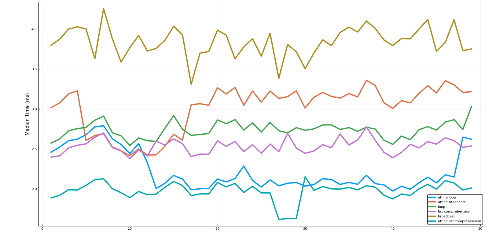
The benchmarked median time for each method ploted against the speech samples
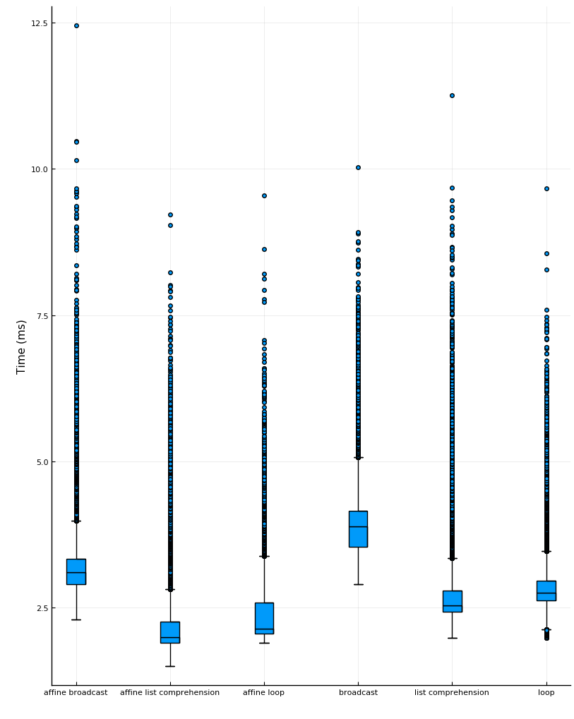
Box plots of the benchmarked time for each method on the samples from the speech library
It is worth noting that all of the tested methods outperform the preexisting implementation which had redundant loops for memory allocation and variable assignment.
4.2 Results
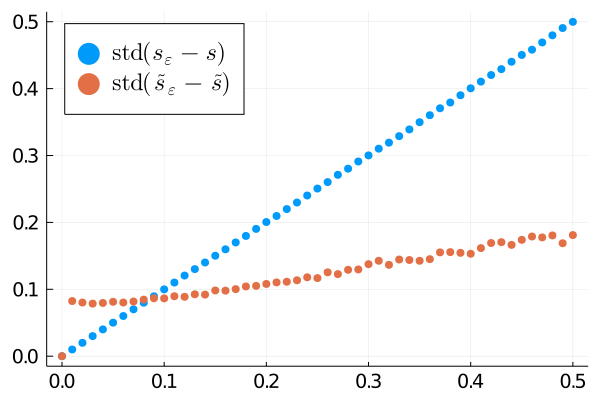
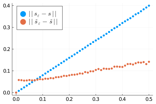
Distance of noisy sound to original one before (blue) and after (red) the processing, plotted against the standard deviation of the noise (\(\varepsilon\)). Left: standard deviation metric. Right: \(\left\lVert\cdot\right\rVert\) norm.
In the figure above, we present the results of the algorithm applied to a denoising task. Namely, given a sound signal \(s\), we let \(s_\varepsilon= s + g_\varepsilon\), where \(g_\varepsilon\sim \mathcal N(0,\varepsilon)\) is a gaussian random variable. We then apply the proposed sound processing algorithm to obtain \(\tilde s_\varepsilon\). As a reconstruction metric we present both the norm \(\left\lVert\cdot\right\rVert\) where for a real signal \(s\), \(\left\lVert s\right\rVert = \left\lVert s\right\rVert_1/\dim(s)\) with \(\left\lVert\cdot\right\rVert_1\) as the \(L_1\) norm and the standard deviation \(\mathrm{std}(\tilde s_\varepsilon -\tilde s)\). We observe that according to both metrics the algorithm indeed improves the signal [4].