1 Background

The focus of this project is music information retrieval from music audio signals. In this section we go through the main problems in the discipline of Automatic Music Transcription, we study characteristics of musical elements, human perception of music, and basic notions of modern music theory. We also review the main characteristics of a sound wave as well as analytic tools for processing digital audio signals. Furthermore, we establish the bridge between music theory and physical properties of audio signals.

1.1 Automatic Music Transcription

AMT is the process of converting an acoustic musical signal into some form of musical notation. (Benetos et al. 2013)

1.1.1 History and community

The interest in the task of AMT has started in the late 20^th century, with researchers borrowing and adapting concepts from the well-established domain of speech-processing. Major strides have been made in the 21^st century, particularly since the creation of the International Society for Music Information Retrieval (ISMIR) in 2000. Which have connected the community and provided a platform for sharing and learning Music Information Retrieval (MIR) concepts worldwide. (Müller 2015)

furthermore, the Music Information Retrieval Evaluation eXchange (MIREX) is an annual evaluation compaign for MIR algorithms. Since it started in 2005, MIREX has served as a benchmark for evaluating novelty algorithms and helped advance MIR Research.

1.1.2 Motivation

MIR and AMT can be of great interest for different demographics. First, most musicians stand to benefit from reliable transcription algorithms as it can facilitate their tasks in difficult cases or for the least accelerate the process.

Moreover, in many music genres such as Jazz, musical notation is rarely used, therefore the exchange formats are almost exclusively recordings of performances. AMT would play a role in democratizing no-score music for new learners and provide an easier canonical format for exchanging music.

Another use of MIR is score-following software development that include a cursor that follows real-time playing indicating the correct and incorrect notes played helping pupils practice and progress on their own more efficiently, making the task of music learning less painful.

Furthermore, MIR allows performing musicological analysis directly on recordings, gaining access to much larger databases compared to anotated music, which can also be applied for various tasks such as music recognition or melody recognition.

1.1.3 Underlying tasks

Automatic Music Transcription is divided into several subtasks where each represents a research topic that fall within the scope of Musical Information Retrieval.

The largest topic of MIR is tonal analysis, which is based on analysing spectral features of audio signals, and subsequently estimating pitch, melody and harmony. Despite the large interest in this topic and various techniques applied, this task remains the core problem in AMT, Exploration of main pitch analysis techniques is the first part of this project.

Another main AMT task is temporal segmentation, which relates consequently to rythme extraction and tempo detection in melodic sounds. (Benetos et al. 2013) This task pertains pertains to spectral features as well as signal energy. We expore this topic in the second part of this project.

Several more tasks are needed to fully transcribe a musical piece, including: loudness estimation, instrument recognition, rhythm detection, scale detection and harmony analysis. In the scope of this project, we limit our study to pitch analysis and temporal segmentation.

1.2 Physical definition of acoustic waves

Sound is generated by vibrating objects, these vibrations cause oscillations of molecules in the medium. The varying pressure propagates through the medium as a wave, the pressure is therefore the solution of the wave equation in time and space, also known as the acoustic wave equation. (Feynman 1965) \[\Delta p =\frac{1}{c^2}\frac{\partial^2 p}{ {\partial t}^2}\] where \(p\) is the accoustic pressure function of time and space and \(c\) is the speed of sound propagation. The wave equation can be solved analytically with the separation of variables method, resulting in a sinusoidal harmonic solutions.

In audio signal processing, we are interested in the pressure at the receptor’s position (listener or microphone), hence the pressure as a function of time. An audio signal is therefore defined as the deviation of pressure from the average pressure of the medium at the receptor’s position.

The pressure function being harmonic, the sound signal is of the form \[\tilde{x}(t) = \sum_{h=0}^{\infty} A_h \cos(2\pi hf_0t + \varphi_h)\] where

• \(f_0\) is called the fundamental frequency of the signal,
• \(h\) is the harmonic number,
• \(A_h\) is the amplitude of the \(h^\text{th}\) harmonic,
• \(\varphi_h\) is the phase of the \(h^\text{th}\) harmonic.

In many works this formula appears in terms of the angular frequency \(\omega=2\pi f\), we denote as well \(f_h = h f_0\) for \(h\geq 1\).

As harmonics represent proper multiples of the fundamental frequency, \(h=0\) is excluded from the sum \[\tilde{x}(t) = a_0 + \sum_{h=1}^{\infty} A_h \cos(2\pi hf_0t + \varphi_h)\] with \(a_0 = A_0\cos(\varphi_0)\).

1.3 Perception of sound and music

The human auditory system is capable of distinguishing intensities and frequencies of sound waves as well as temporal features. The inner ear is extremely sensitive to sound wave features, the brain allows further analysis of these features.

Music theory defines and studies perceived features of music signals. These features are based on the signal’s intensity, frequency, and time patterns.

In music theory, a note is a musical symbol that represents the smallest musical object. The note’s attributes define the pitch of the sound, its relative duration and its relative intensity.

1.3.1 Fundamental frequency and pitch

Sound signals are periodic, therefore by definition there exists a \(T>0\) such as \[\forall t, \tilde{x}(t)=\tilde{x}(t+T)\] which follows that there exists an infinite set of values of \(T>0\) that verify this property, indeed \(\forall n\in\mathbb{N}, T'=nT, \tilde{x}(t)=\tilde{x}(t+T')\). We define the period of a signal as the smallest positive value of \(T\) for which the property holds. The fundamental frequency \(f_0\) is defined formally as the reciprocal of the period. This definition holds for any periodic signal, regardless of its form.

In the case of sound wave, the perception of the fundamental frequency is referred to as the pitch. Pitch is the defined as the tonal height of a sound, it is closely related to the fundamental frequency however remaining a relative musical concept unlike the \(f_0\) of a signal that is an absolute mathematical value. In fact, the relation between pitch and \(f_0\) is neither bijective nor invariant.

In music theory, pitch is defined on a discrete space unlike the continuous frequency space. Moreover, human perception of frequency is logarithmic hence obtaining the next pitch corresponds to the multiplication of the frequency by a certain value \(r\).

Finally, the frequency of the reference pitch A₄ is widely accepted today as \(440 Hz\) while in the baroque era it was around \(415 Hz\) and \(440 Hz\) was the frequency corresponding to A♯ pitch. Even in modern day, variations of the pitch frequency exist in different regions and even different orchestras!

1.3.2 Perception of intensity

Sound intensity is defined physically as the power carried by sound waves per unit area, whereas sound pressure is the local pressure deviation from the ambient atmospheric pressure caused by a sound wave. Human perception of intensity is directly sensitive to sound pressure, it is measured in terms of sound pressure level (SPL) which is a logarithmic measure of sound pressure \(P\) relative to the atmospheric pressure \(P_0\) measured in decibels \(\mathrm{dB}\). \[\mathrm{SPL} = 20\log_{10}\left(\frac{P}{P_0}\right) \mathrm{dB}\]

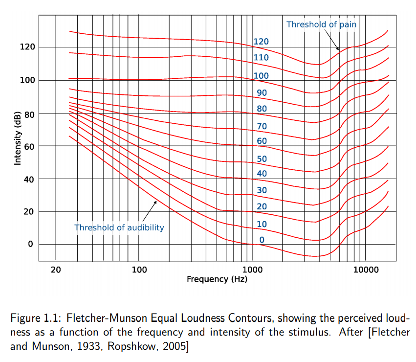
Nevertheless, sensitivity to sound intensity is variable across different frequencies. The subjective perception of sound pressure is defined by a sound’s loudness which is a function of both SPL and frequency ranging from quiet to loud.

In music theory, loudness is defined by a piece’s dynamics. Dynamics are indicators of a part’s loudness relative to other parts and/or instruments. Dynamics markings are expressed with the italian keywords forte \(\boldsymbol{f}\) (loud) and piano \(\boldsymbol{p}\) (soft). Subtle degrees of loudness can be expressed by the prefixes mezzo- or più, for example \(\boldsymbol{mp}\) stands for mezzo-piano (moderately soft) and \(pi\grave{u}~\boldsymbol{p}\) (softer), or by consecutive letters such as fortissimo \(\boldsymbol{f}\hspace{-2pt}\boldsymbol{f}\) (very loud) or more letters if needed.

Music dynamics also allow expressing gradual changes in loudness, indicated as symbols or italian keywords (crescendo and diminuendo).

1.4 Audio signal processing

1.4.1 Discrete-time signals

The domain of audio signal processing deals with recorded digital/analog signals, which are discrete-time signals. The Nyquist-Shannon sampling theorem is the fundamental bridge between continuous-time and discrete-time signals. It establishes a sufficient condition for a sample rate that permits a discrete sequence of samples to capture all the information from a continuous-time signal. (Wikipedia 2020)

The sample rate \(f_s\) of a discrete-time signal is defined as the number of samples per second, its inverse is the time step between samples \(T_s\).

We denote, conformely to litterature a discrete signal time frame as \(x[n]=x(t_n)\) where \(t_n=n\cdot T_s=\frac{n}{f_s}\).

1.4.2 Discrete Fourier Transform (DFT)

The discrete Fourier transform of \(N\) samples, with a sample rate of \(f_s\) can be obtained from its continuous definition.

\[\begin{align} X(f) &= \int\limits_{0}^{t_N} x(t)\cdot e^{-2\pi j ft}\mathrm{d}t\\ &= \lim\limits_{f_s\rightarrow\infty} \sum\limits_{n=0}^{N-1} x(t_n)\cdot e^{-2\pi j ft_n}\\ &= \lim\limits_{f_s\rightarrow\infty} \underbrace{\sum\limits_{n=0}^{N-1} x[n]\cdot e^{-2\pi j f \frac{n}{f_s}}}_{X[f]}\\ &= \lim\limits_{f_s\rightarrow\infty} X[f] \end{align}\]

The DFT of \(x[n]\) is given for all frequency bins \(k=0,\ldots,K\) \[X[k] = \sum\limits_{n=0}^{N-1} x[n]\cdot e^{-2\pi j k \frac{n}{f_s}}\]

References

Benetos, Emmanouil, Simon Dixon, Dimitrios Giannoulis, Holger Kirchhoff, and Anssi Klapuri. 2013. “Automatic Music Transcription: Challenges and Future Directions.” Journal of Intelligent Information Systems 41 (December). https://doi.org/10.1007/s10844-013-0258-3.

Feynman, Richard. 1965. “The Feynman Lectures on Physics Vol. I Ch. 47: Sound. The Wave Equation.” https://www.feynmanlectures.caltech.edu/I_47.html.

Müller, Meinard. 2015. Fundamentals of Music Processing - Audio, Analysis, Algorithms, Applications. Springer. https://www.audiolabs-erlangen.de/fau/professor/mueller/bookFMP.

Wikipedia. 2020. “Nyquist–Shannon Sampling Theorem.” Wikipedia. https://en.wikipedia.org/w/index.php?title=Nyquist%E2%80%93Shannon_sampling_theorem&oldid=941933031.